Machine-code instructions

Algorithm 2.4 may seem artificial, but it a faithful representation of the actual im- plementation of computer programs. Programs written in a programming language like Ada or Java are compiled into machine code. In some cases, the code is for a specific processor, while in other cases, the code is for a virtual machine like the Java Virtual Machine (JVM). Code for a virtual machine is then interpreted or a further compilation step is used to obtain code for a specific processor. While there are many different computer architectures—both real and virtual—they have much in common and typically fall into one of two categories.

Register machines

A register machine performs all its computations in a small amount of high-speed memory called registers that are an integral part of the CPU. The source code of the program and the data used by the program are stored in large banks of memory, so that much of the machine code of a program consists of load instructions, which move data from memory to a register, and store instructions, which move data from a register to memory. load and store of a memory cell (byte or word) is atomic.

The following algorithm shows the code that would be obtained by compiling Algorithm 2.3 for a register machine:

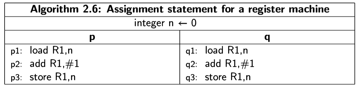
The notation add R1, #1 means that the value 1 is added to the contents of register R1, rather than the contents of the memory cell whose address is 1.

The following diagram shows the execution of the three instructions:

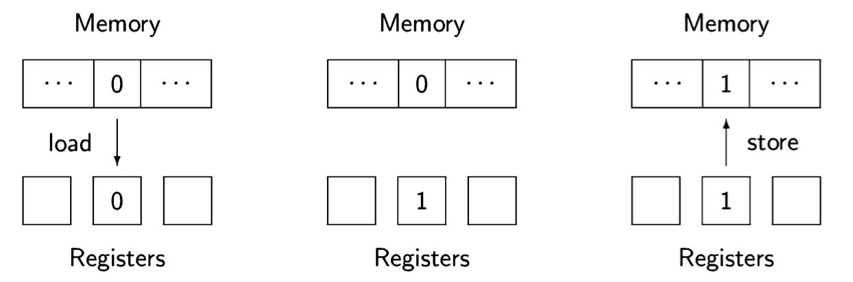
First, the value stored in the memory cell for n is loaded into one of the registers; second, the value is incremented within the register; and third, the value is stored back into the memory cell.

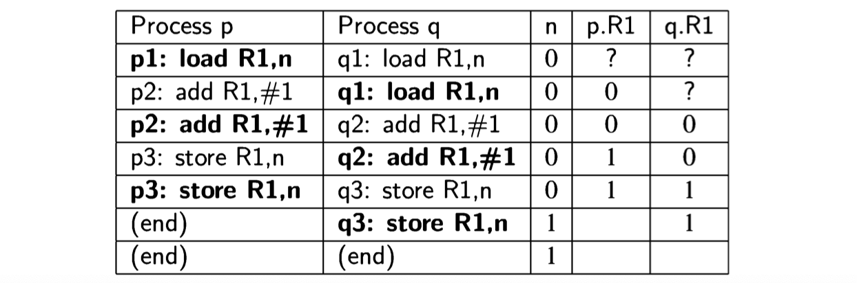
Ostensibly, both processes are using the same register R1, but in fact, each process keeps its own copy of the registers. This is true not only on a multiprocessor or distributed system where each CPU has its own set of registers, but even on a multitasking single-CPU system, as described in Section 2.3. The context switch mechanism enables each process to run within its own context consisting of the current data in the computational registers and other registers such as the control pointer. Thus we can look upon the registers as analogous to the local variables temp in Algorithm 2.4 and a bad scenario exists that is analogous to the bad scenario for that algorithm:

Stack machines

The other type of machine architecture is the stack machine. In this architecture, data is held not in registers but on a stack, and computations are implicitly performed on the top elements of a stack. The atomic instructions include push and pop, as well as instructions that perform arithmetical, logical and control operations on elements of the stack. In the register machine, the instruction add R1,#1 explicitly mentions its operands, while in a stack machine the instruction would simply be written add, and it would add the values in the top two positions in the stack, leaving the result on the top in place of the two operands:

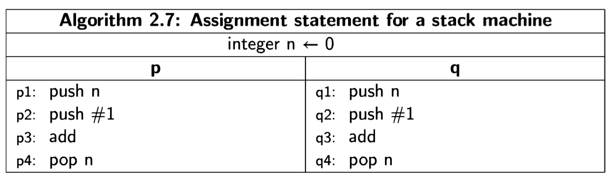
The following diagram shows the execution of these instructions on a stack machine:

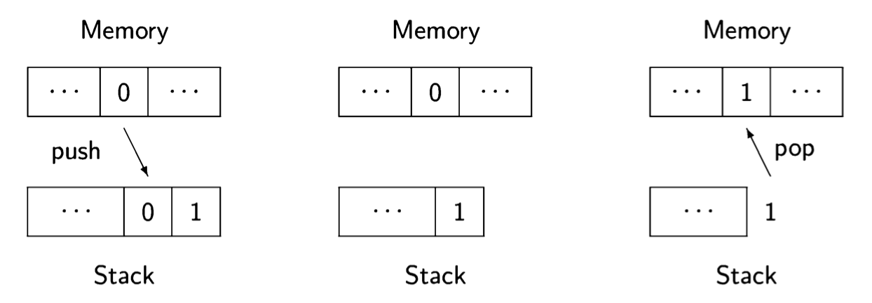
Initially, the value of the memory cell for n is pushed onto the stack, along with the constant 1. Then the two top elements of the stack are added and replaced by one element with the result. Finally (on the right), the result is popped off the stack and stored in the memory cell. Each process has its own stack, so the top of the stack, where the computation takes place, is analogous to a local variable.

It is easier to write code for a stack machine, because all computation takes place in one place, whereas in a register machine with more than one computational register you have to deal with the allocation of registers to the various operands. This is a non-trivial task that is discussed in textbooks on compilation. Furthermore, since different machines have different numbers and types of registers, code for register machines is not portable. On the other hand, operations with registers are extremely fast, whereas if a stack is implemented in main memory access to operands will be much slower.

For these reasons, stack architectures are common in virtual machines where sim- plicity and portability are most important. When efficiency is needed, code for the virtual machine can be compiled and optimized for a specific real machine. For our purposes the difference is not great, as long as we have the concept of memory that may be either global to all processes or local to a single process. Since global and local variables exist in high-level programming languages, we do not need to discuss machine code at all, as long as we understand that some local variables are being used as surrogates for their machine-language equivalents.

Source statements and machine instructions

We have specified that source statements like

are atomic. As shown in Algorithm 2.6 and Algorithm 2.7, such source statements must be compiled into a sequence of machine language instructions. (On some computers n<-n+1 can be compiled into an atomic increment instruction, but this is not true for a general assignment statement.) This increases the number of interleavings and leads to incorrect results that would not occur if the source statement were really executed atomically.

However, we can study concurrency at the level of source statements by decompos- ing atomic statements into a sequence of simpler source statements. This is what we did in Algorithm 2.4, where the above atomic statement was decomposed into the pair of statements:

The concept of a simple source statement can be formally defined:

Definition 2.7 An occurrence of a variable v is defined to be critical reference: (a) if it is assigned to in one process and has an occurrence in another process, or (b) if it has an occurrence in an expression in one process and is assigned to in another.

A program satisfies the limited-critical-reference (LCR) restriction if each statement contains at most one critical reference.

Consider the first occurrence of n in \(n \leftarrow n + 1\). It is assigned to in process p and has (two) occurrences in process q, so it is critical by (a). The second occurrence of n in \(n \leftarrow n + 1\) is critical by (b) because it appears in the expression \(n+1\) in p and is also assigned to in q. Consider now the version of the statements that uses local variables. Again, the occurrences of n are critical, but the occurrences of temp are not. Therefore, the program satisfies the LCR restriction. Concurrent programs that satisfy the LCR restriction yield the same set of behaviors whether the statements are considered atomic or are compiled to a machine architecture with atomic load and store. See [50, Section 2.2] for more details.

The more advanced algorithms in this book do not satisfy the LCR restriction, but can easily be transformed into programs that do satisfy it. The transformed programs may require additional synchronization to prevent incorrect scenarios, but the additions are simple and do not contribute to understanding the concepts of the advanced algorithms.