Concurrent execution as interleaving of atomic statements

We now define the concurrent programming abstraction that we will study in this textbook. The abstraction is based upon the concept of a (sequential) process, which we will not formally define. Consider it as a normal program fragment written in a programming language. You will not be misled if you think of a process as a fancy name for a procedure or method in an ordinary programming language.

Definition 2.1 A concurrent program consists of a finite set of (sequential) pro- cesses. The processes are written using a finite set of atomic statements. The execution of a concurrent program proceeds by executing a sequence of the atomic statements obtained by arbitrarily interleaving the atomic statements from the pro- cesses. A computation is an execution sequence that can occur as a result of the interleaving. Computations are also called scenarios.

Definition 2.2 During a computation the control pointer of a process indicates the next statement that can be executed by that process. Each process has its own control pointer.

Computations are created by interleaving, which merges several statement streams. At each step during the execution of the current program, the next statement to be executed will be chosen from the statements pointed to by the control pointers cp of the processes.

Suppose that we have two processes, p composed of statements \(p1\) followed by \(p2\) and \(q\) composed of statements \(q1\) followed by \(q2\), and that the execution is started with the control pointers of the two processes pointing to \(p1\) and \(q1\). Assuming that the statements are assignment statements that do not transfer control, the possible scenarios are:

\[ p1 \rightarrow q1 \rightarrow p2 \rightarrow q2, \] \[ p1 \rightarrow q1 \rightarrow q2 \rightarrow p2, \] \[ p1 \rightarrow p2 \rightarrow q1 \rightarrow q2, \] \[ q1 \rightarrow p1 \rightarrow q2 \rightarrow p2, \] \[ q1 \rightarrow p1 \rightarrow p2 \rightarrow q2, \] \[ q1 \rightarrow q2 \rightarrow p1 \rightarrow p2. \]

Note that \(p2 \rightarrow p1 \rightarrow q1 \rightarrow q2 \) is not a scenario, because we respect the sequential execution of each individual process, so that \(p2\) cannot be executed before \(p1\).

We will present concurrent programs in a language-independent form, because the concepts are universal, whether they are implemented as operating systems calls, directly in programming languages like Ada or Java, or in a model specification language like Promela. The notation is demonstrated by the following trivial two- process concurrent algorithm:

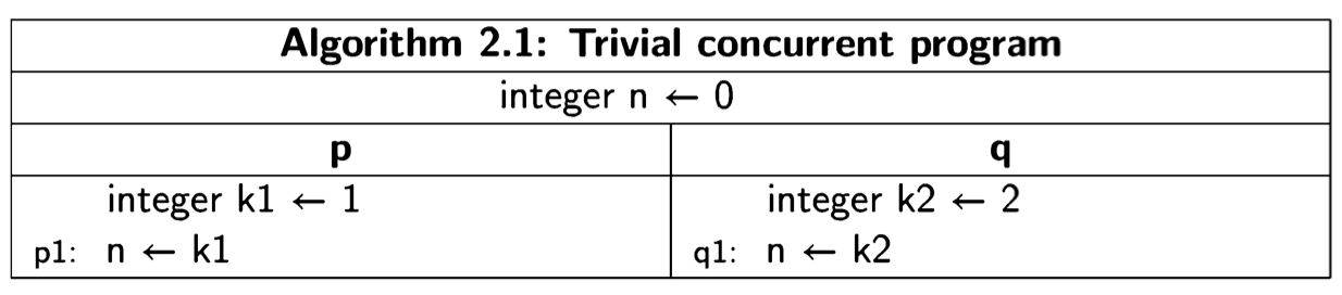
The program is given a title, followed by declarations of global variables, followed by two columns, one for each of the two processes, which by convention are named process p and process q. Each process may have declarations of local variables, followed by the statements of the process. We use the following convention:

States

The execution of a concurrent program is defined by states and transitions between states. Let us first look at these concepts in a sequential version of the above algorithm:

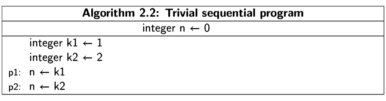
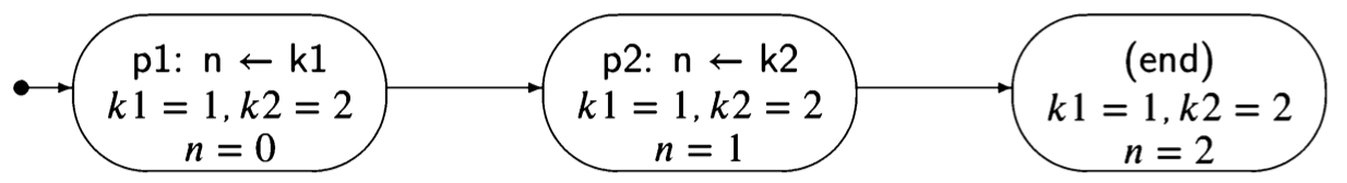
At any time during the execution of this program, it must be in a state defined by the value of the control pointer and the values of the three variables. Executing a statement corresponds to making a transition from one state to another. It is clear that this program can be in one of three states: an initial state and two other states obtained by executing the two statements. This is shown in the following diagram, where a node represents a state, arrows represent the transitions, and the initial state is pointed to by the short arrow on the left:

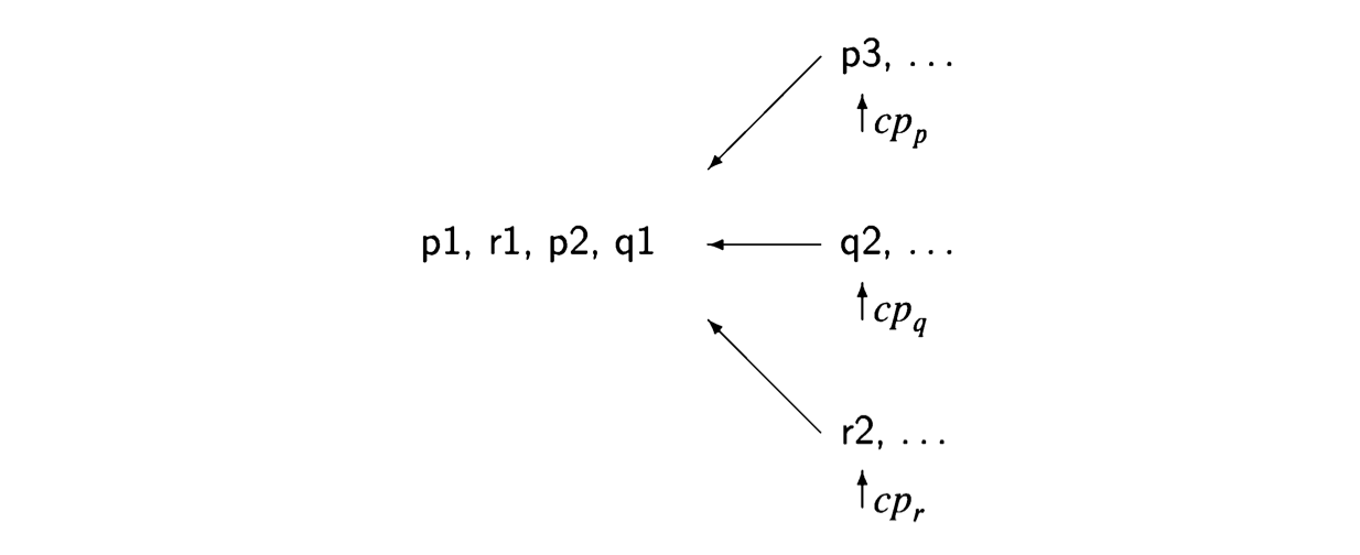
Consider now the trivial concurrent program Algorithm 2.1 There are two pro- cesses, so the state must include the control pointers of both processes. Further- more, in the initial state there is a choice as to which statement to execute, so there are two transitions from the initial state.

The lefthand states correspond to executing p1 followed by q1, while the righthand states correspond to executing q1 followed by pl. Note that the computation can terminate in two different states (with different values of 1), depending on the interleaving of the statements.

Definition 2.3 The state of a (concurrent) algorithm is a tuple consisting of one element for each process that is a label from that process, and one element for each global or local variable that is a value whose type is the same as the type of the variable.

The number of possible states—the number of tuples—is quite large, but in an execution of a program, not all possible states can occur. For example, since no values are assigned to the variables k1 and k2 in Algorithm 2.1, no state can occur in which these variables have values that are different from their initial values.

Definition 2.4 Let \(s_1\) and \(s_2\) be states. There is a transition between \(s_1\), and \(s_2\) if executing a statement in state \(s_1\) changes the state to \(s_2\). The statement executed must be one of those pointed to by a control pointer in \(s_1\).

Definition 2.5 A state diagram is a graph defined inductively. The initial state diagram contains a single node labeled with the initial state. If state \(s_1\) labels a node in the state diagram, and if there is a transition from \(s_1\) to \(s_2\), then there is a node labeled \(s_2\) in the state diagram and a directed edge from \(s_1\) to \(s_2\).

For each state, there is only one node labeled with that state.

The set of reachable states is the set of states in a state diagram.

It follows from the definitions that a computation (scenario) of a concurrent pro- gram is represented by a directed path through the state diagram starting from the initial state, and that all computations can be so represented. Cycles in the state diagram represent the possibility of infinite computations in a finite graph.

The state diagram for Algorithm 2.1 shows that there are two different scenarios, each of which contains three of the five reachable states.

Scenarios

A scenario is defined by a sequence of states. Since diagrams can be hard to draw, especially for large programs, it is convenient to use a tabular representation of scenarios. This is done simply by listing the sequence of states in a table; the columns for the control pointers are labeled with the processes and the columns for the variable values with the variable names. The following table shows the scenario of Algorithm 2.1 corresponding to the lefthand path:

In a state, there may be more than one statement that can be executed. We use bold font to denote the statement that was executed to get to the state in the following row.